Baseball Analytics: An Introduction to Sabermetrics using Python

Sabermetrics is the apllication of statistical analysis to baseball data in order to measure in-game activity. The term Sabermetrics comes from saber (Society for American Baseball Research) and metrics (as in econometrics).

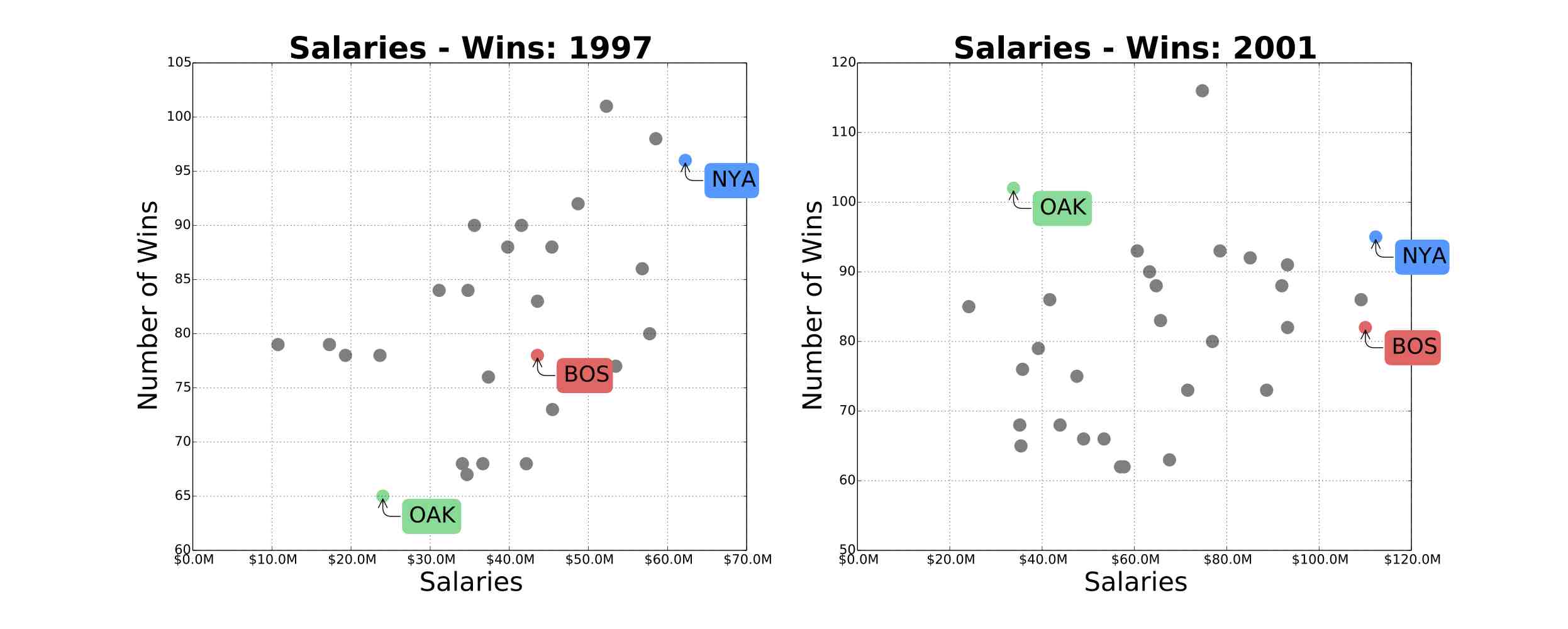
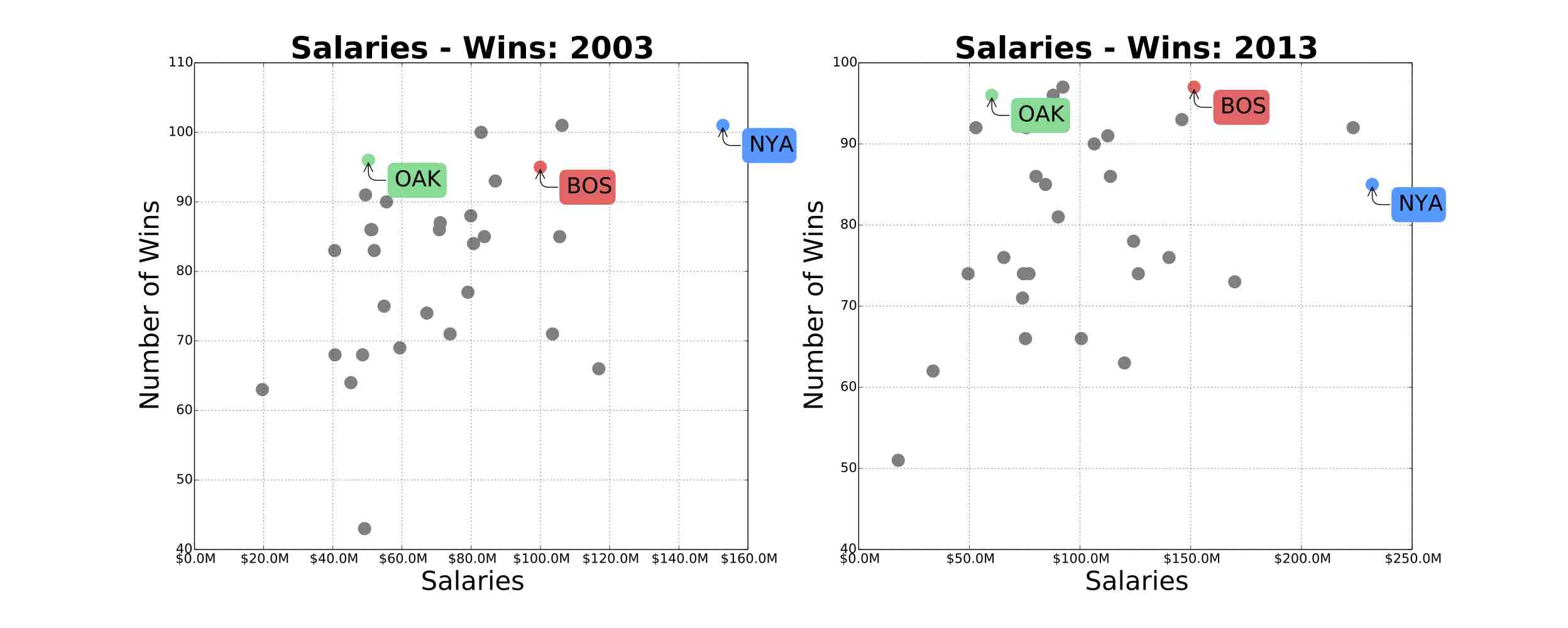
In 2003, Michael Lewis published Moneyball about Billy Beane, the Oakland Athletics General Manager since 1997. The book was centered around Billy Beane's use of Sabemetrics to identify and recruit under-valued baseball players. With this strategy, his team could achieve as many wins as teams with more than double the payroll. The figures below show the relationship between team salaries and number of wins for years: 1997, 2001, 2003, 2013. The green dot represents the Oakland Athletics, the blue dot represents the New York Yankees, and the red dot represents The Boston Red Sox. We can see that the Oakland Athletics went from the underperforming team in 1997, to became a highly competitive team with a comparable number of wins to the New York Yankees. The Oakland Athletics made it to the play-offs in 4 successive years: 2000,2001,2002,2003.

In 2011, the movie Moneyball based on Lewis' book was released starring Brad Pitt in the role of Beane.

In this post, I will use Lahman’s Baseball Database and Python programming language to explain some of the techniques used in Sabermetrics. I will use 3 Python libraries: Pandas for data manipulation and analysis, statsmodels for building the statistical models and Matplotlib for data visualization.

1. A quick introduction to baseball rules

2. Getting the data and setting up your machine

For this tutorial, we will use the Lahman’s Baseball Database. This Database contains complete batting and pitching statistics from 1871 to 2013, plus fielding statistics, standings, team stats, managerial records, post-season data, and more. You can download the data from this this link. We will be using two files from this dataset: Salaries.csv and Teams.csv. To execute the code from this tutorial, you will need Python 2.7 and the following Python Libraries: Numpy, Scipy, Pandas and Matplotlib and statsmodels.

3. Reading and understading the data

We will start by importing the required libraries using the commands below:

import pandas as pd
import scipy as sp
import matplotlib.pyplot as plt
from matplotlib.ticker import FuncFormatter

Next, we will read the Teams.csv file to a Pandas DataFrame called teams. This file contains teams statistics from 1871 to 2013. The dataset has 2745 data points. Each data point has 48 attributes.

teams = pd.read_csv('../data/Teams.csv')

Next, we will select a subset of the data starting from 1985, with 15 Attributes only. For the remaining of this tutorial we will use only this subset and throw the rest of the data.

teams = teams[teams['yearID'] >= 1985]
teams = teams[['yearID', 'teamID', 'Rank', 'R', 'RA', 'G', 'W', 'H', 'BB', 'HBP', 'AB', 'SF', 'HR', '2B', '3B']]

Below is an explanation of the teams DataFrame attribtues.

• yearID: Year
• teamID: Team
• Rank: Position in final standings
• R: Runs scored
• RA: Opponents runs scored
• G: Games played
• W: Wins
• H: Hits by batters
• BB: Walks by batters
• HBP: Batters hit by pitch
• AB: At bats
• SF: Sacrifice flies
• HR: Homeruns by batters
• 2B: Doubles
• 3B: Triples

Next, we will change the teams DataFrame index to ('yearID', 'teamID').

teams = teams.set_index(['yearID', 'teamID'])

This index change will make our queries easier. For example, we can check the number of wins by the Oakland Athletics in 2001 by running the command below. This should return 102.

teams['W'][2001, 'OAK']

Next, we will read the Salaries.csv to a Pandas DataFrame called salaries. The salaries DataFrame contains the salaries of all baseball players from 1985 till 2013. The DataFrame has 5 columns: yearID, teamID, lgID, playerID, salary.

salaries = pd.read_csv('../data/Salaries.csv')

We are interested in calculating baseball teams payroll. We can do so by running the command below.

salaries_by_yearID_teamID = salaries.groupby(['yearID', 'teamID'])['salary'].sum()

Now we can check the payroll of the Oakland Athletics in 2001 by running the command below. This should return 33810750.

salaries_by_yearID_teamID[2001, 'OAK']

Next, we will add the payroll data to teams DataFrame. We can do so using the command below.

teams = teams.join(salaries_by_yearID_teamID)

The payroll data is now stored in a column called salary. Now we can check the payroll of the Oakland Athletics in 2001 by running the command below.

teams['salary'][2001, 'OAK']

Next we will plot the relationship between salaries and number of wins. We can do so for the year 2001 by using the command below.

plt.plot(teams['salary'][2001], teams['W'][2001])
plt.show()

The following two functions are used to plot the relationship between salaries with labels and axis formating; as well as highlighting the Oakland Athletics, the New York Yankees, and the Boston Red Sox data.

def millions(x, pos):
    'The two args are the value and tick position'
    return '$%1.1fM' % (x*1e-6)

formatter = FuncFormatter(millions)

def plot_spending_wins(teams, year):    
    teams_year = teams.xs(year)
    fig, ax = plt.subplots()
    for i in teams_year.index:
        if i == 'OAK':
            ax.scatter(teams_year['salary'][i], teams_year['W'][i], color="#4DDB94", s=200)
            ax.annotate(i, (teams_year['salary'][i], teams_year['W'][i]),
                        bbox=dict(boxstyle="round", color="#4DDB94"),
                        xytext=(-30, 30), textcoords='offset points',
                        arrowprops=dict(arrowstyle="->", connectionstyle="angle,angleA=0,angleB=90,rad=10"))
        elif i == 'NYA':
            ax.scatter(teams_year['salary'][i], teams_year['W'][i], color="#0099FF", s=200)
            ax.annotate(i, (teams_year['salary'][i], teams_year['W'][i]),
                        bbox=dict(boxstyle="round", color="#0099FF"),
                        xytext=(30, -30), textcoords='offset points',
                        arrowprops=dict(arrowstyle="->", connectionstyle="angle,angleA=0,angleB=90,rad=10"))
        elif i == 'BOS':
            ax.scatter(teams_year['salary'][i], teams_year['W'][i], color="#FF6666", s=200)
            ax.annotate(i, (teams_year['salary'][i], teams_year['W'][i]),
                        bbox=dict(boxstyle="round", color="#FF6666"),
                        xytext=(-30, 30), textcoords='offset points',
                        arrowprops=dict(arrowstyle="->", connectionstyle="angle,angleA=0,angleB=90,rad=10"))     
        else:
            ax.scatter(teams_year['salary'][i], teams_year['W'][i], color="grey", s=200)
    ax.xaxis.set_major_formatter(formatter) 
    ax.tick_params(axis='x', labelsize=15)
    ax.tick_params(axis='y', labelsize=15)
    ax.set_xlabel('Salaries', fontsize=20)
    ax.set_ylabel('Number of Wins' , fontsize=20)
    ax.set_title('Salaries - Wins: '+ str(year), fontsize=25, fontweight='bold')
    plt.show()

We can run the plot_spending_wins by passing the teams DataFrame and the year variable. For example, for plotting 2001 salaries and number of wins relationship, we execute the following:

plot_spending_wins(teams, 2001)

4. Bill Beane's Formula

For a Baseball team to win a game, it needs to score more runs than it allows. In the remaining of this tutorial, we will build a mathematical model for runs scored. Similar logic could be applied for modelling runs allowed.

Most teams focused on Batting Average (BA) as a statistic to improve their runs Scored. Bill Beane took a different approach, he focused on improving On Base Percentage (OBP), and Slugging Percentage (SLG).

The Batting Average is defined by the number of hits divided by at bats. It can be calculated using the formula below:

On-base Percentage is a measure of how often a batter reaches base for any reason other than a fielding error, fielder's choice, dropped/uncaught third strike, fielder's obstruction, or catcher's interference. It can be calculated using the formula below:

Slugging Percentage is a measure of the power of a hitter. It can ve calculated using the formula below:

We will add these 3 measures to our teams DataFrame by running the following commands:

teams['BA'] = teams['H']/teams['AB']
teams['OBP'] = (teams['H'] + teams['BB'] + teams['HBP']) / (teams['AB'] + teams['BB'] + teams['HBP'] + teams['SF'])
teams['SLG'] = (teams['H'] + teams['2B'] + (2*teams['3B']) + (3*teams['HR'])) / teams['AB']

Next, we will use a linear regression model to verify which baseball stats are more important to predict runs. We will build 3 different models: The first one will have as features OBP, SLG and BA. The second model will have as features OBP and SLG. The last one will have as feature BA only.

We will use Python's statsmodels library for building these models. We start first by importing the library by running:

import statsmodels.formula.api as sm

Next we will build our models:

#First Model
runs_reg_model1 = sm.ols("R~OBP+SLG+BA",teams)
runs_reg1 = runs_reg_model1.fit()
#Second Model
runs_reg_model2 = sm.ols("R~OBP+SLG",teams)
runs_reg2 = runs_reg_model2.fit()
#Third Model
runs_reg_model3 = sm.ols("R~BA",teams)
runs_reg3 = runs_reg_model3.fit()

We can look at a summary statistic of these models by running:

runs_reg1.summary()
runs_reg2.summary()
runs_reg3.summary()

The first model has an Adjusted R-squared of 0.918, with 95% confidence interval of BA between -283 and 468. This is counterintuitive, since we expect the BA value to be positive. This is due to a multicollinearity between the variables.

The second model has an Adjusted R-squared of 0.919, and the last model an Adjusted R-squared of 0.500.

Based on this analysis, we could confirm that the second model using OBP and SLG is the best model for predicting Run Scored.

Recruting strategy based on Bill Beane's Formula

Based on the analysis above, a good strategy for recruiting batters would focus on targeting undervalued players with high OBP and SLG. In the late 1990s, the old school scouts overvalued BA, and players with high BA had high salaries. Although BA and OBP have a positive correlation, there were some players that have high OBP and SLG, and relatively small BA. These players were undervalued by the market, and were the target of Billy Beane.

5. Conclusion

The techniques and Python code introduced in this tutorial could be extended to build different statistical models and data visualizations.

All the source code and data from this tutorial can be found at this github repo.

References

http://www.swing-smarter-baseball-hitting-drills.com/oakland-as.html

MITx: 15.071x The Analytics Edge