Deep learning is the new big trend in machine learning. It had many recent successes in computer vision, automatic speech recognition and natural language processing.

The goal of this blog post is to give you a hands-on introduction to deep learning. To do this, we will build a Cat/Dog image classifier using a deep learning algorithm called convolutional neural network (CNN) and a Kaggle dataset.

This post is divided into 2 main parts. The first part covers some core concepts behind deep learning, while the second part is structured in a hands-on tutorial format.

In the first part of the hands-on tutorial (section 4), we will build a Cat/Dog image classifier using a convolutional neural network from scratch. In the second part of the tutorial (section 5), we will cover an advanced technique for training convolutional neural networks called transfer learning. We will use some Python code and a popular open source deep learning framework called Caffe to build the classifier. Our classifier will be able to achieve a classification accuracy of 97%.

By the end of this post, you will understand how convolutional neural networks work, and you will get familiar with the steps and the code for building these networks.

The source code for this tutorial can be found in this github repository.

1. Problem Definition

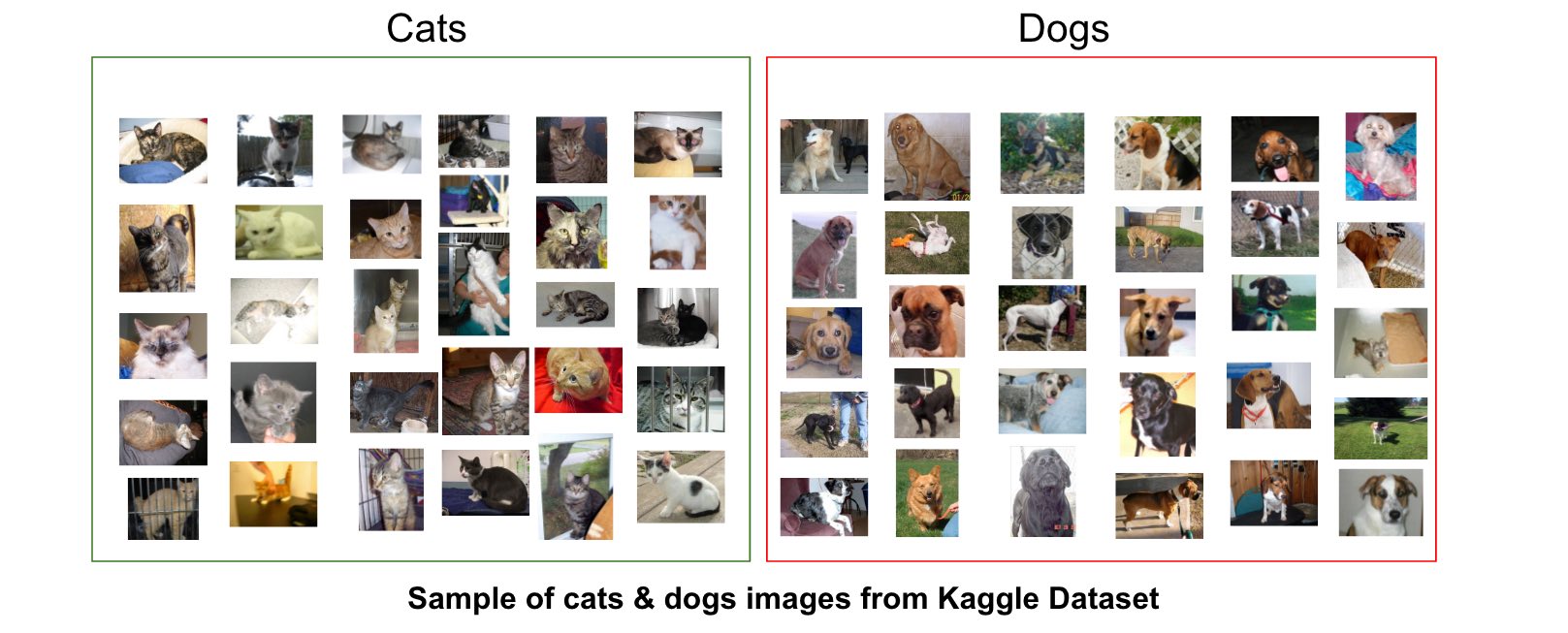
In this tutorial, we will be using a dataset from Kaggle. The dataset is comprised of 25,000 images of dogs and cats.

Our goal is to build a machine learning algorithm capable of detecting the correct animal (cat or dog) in new unseen images.

In Machine learning, this type of problems is called classification.

2. Classification using Traditional Machine Learning vs. Deep Learning

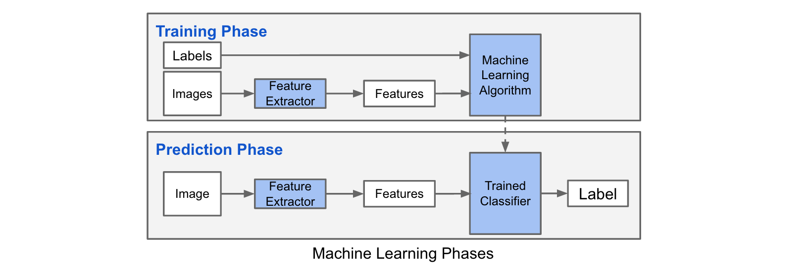
Classification using a machine learning algorithm has 2 phases:

• Training phase: In this phase, we train a machine learning algorithm using a dataset comprised of the images and their corresponding labels.
• Prediction phase: In this phase, we utilize the trained model to predict labels of unseen images.

The training phase for an image classification problem has 2 main steps:

1. Feature Extraction: In this phase, we utilize domain knowledge to extract new features that will be used by the machine learning algorithm. HoG and SIFT are examples of features used in image classification.

2. Model Training: In this phase, we utilize a clean dataset composed of the images' features and the corresponding labels to train the machine learning model.

In the predicition phase, we apply the same feature extraction process to the new images and we pass the features to the trained machine learning algorithm to predict the label.

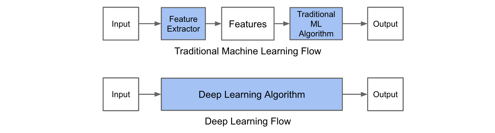
The main difference between traditional machine learning and deep learning algorithms is in the feature engineering. In traditional machine learning algorithms, we need to hand-craft the features. By contrast, in deep learning algorithms feature engineering is done automatically by the algorithm. Feature engineering is difficult, time-consuming and requires domain expertise. The promise of deep learning is more accurate machine learning algorithms compared to traditional machine learning with less or no feature engineering.

3. A Crash Course in Deep Learning

Deep learning refers to a class of artificial neural networks (ANNs) composed of many processing layers. ANNs existed for many decades, but attempts at training deep architectures of ANNs failed until Geoffrey Hinton's breakthrough work of the mid-2000s. In addition to algorithmic innovations, the increase in computing capabilities using GPUs and the collection of larger datasets are all factors that helped in the recent surge of deep learning.

3.1. Artificial Neural Networks (ANNs)

Artificial neural networks (ANNs) are a family of machine learning models inspired by biological neural networks.

Artificial Neural Networks vs. Biological Neural Networks

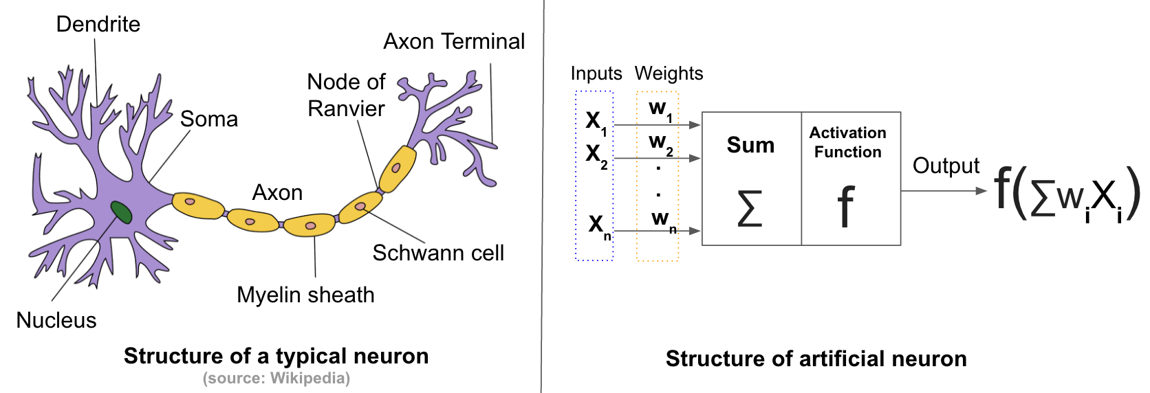
Biological Neurons are the core components of the human brain. A neuron consists of a cell body, dendrites, and an axon. It processes and transmit information to other neurons by emitting electrical signals. Each neuron receives input signals from its dendrites and produces output signals along its axon. The axon branches out and connects via synapses to dendrites of other neurons.

A basic model for how the neurons work goes as follows: Each synapse has a strength that is learnable and control the strength of influence of one neuron on another. The dendrites carry the signals to the target neuron's body where they get summed. If the final sum is above a certain threshold, the neuron get fired, sending a spike along its axon.[1]

Artificial neurons are inspired by biological neurons, and try to formulate the model explained above in a computational form. An artificial neuron has a finite number of inputs with weights associated to them, and an activation function (also called transfer function). The output of the neuron is the result of the activation function applied to the weighted sum of inputs. Artificial neurons are connected with each others to form artificial neural networks.

Feedforward Neural Networks

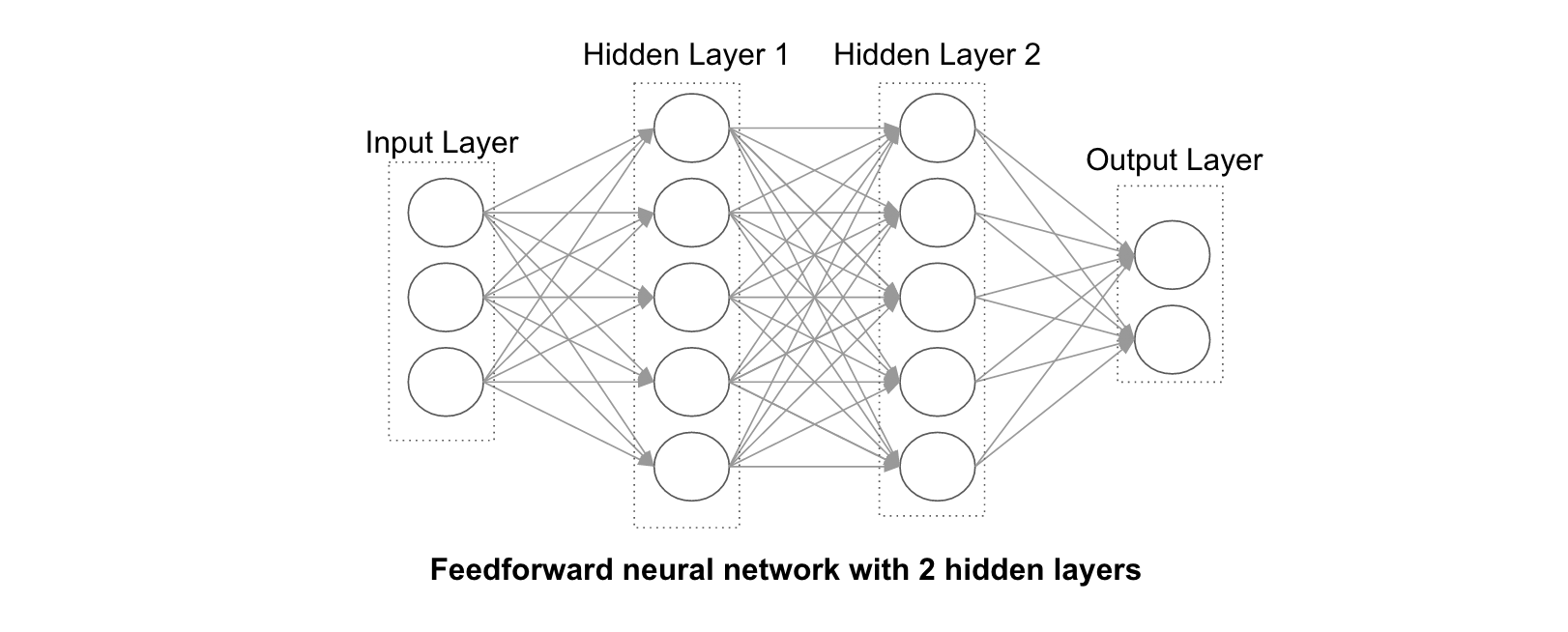
Feedforward Neural Networks are the simplest form of Artificial Neural Networks.

These networks have 3 types of layers: Input layer, hidden layer and output layer. In these networks, data moves from the input layer through the hidden nodes (if any) and to the output nodes.

Below is an example of a fully-connected feedforward neural network with 2 hidden layers. "Fully-connected" means that each node is connected to all the nodes in the next layer.

Note that, the number of hidden layers and their size are the only free parameters. The larger and deeper the hidden layers, the more complex patterns we can model in theory.

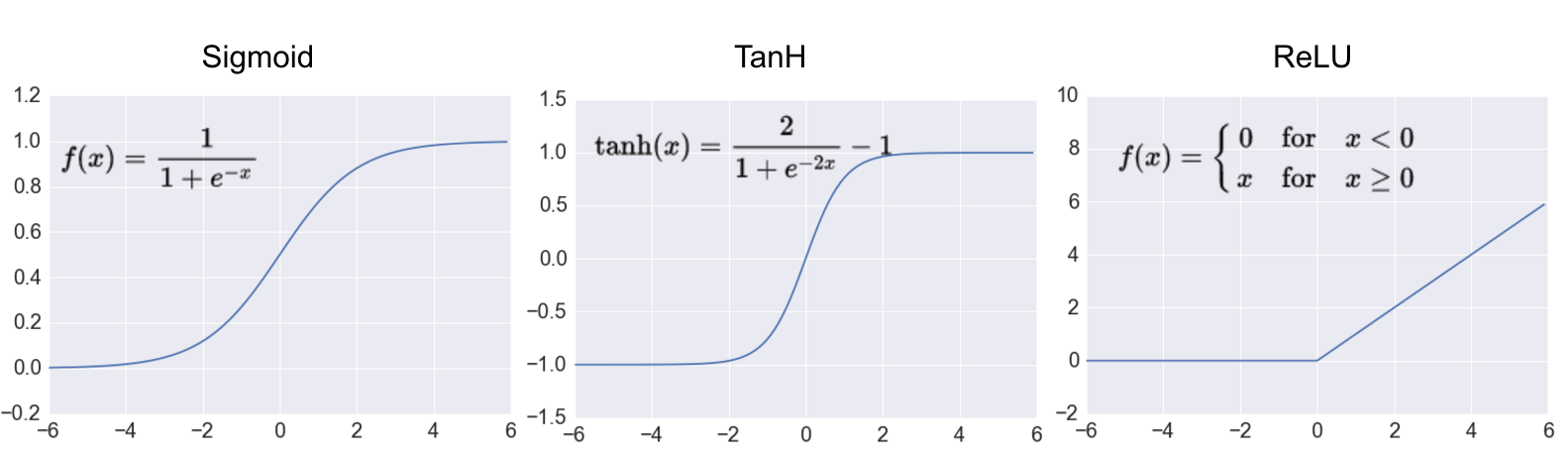
Activation Functions

Activation functions transform the weighted sum of inputs that goes into the artificial neurons. These functions should be non-linear to encode complex patterns of the data. The most popular activation functions are Sigmoid, Tanh and ReLU. ReLU is the most popular activation function in deep neural networks.

Training Artificial Neural Networks

The goal of the training phase is to learn the network's weights. We need 2 elements to train an artificial neural network:

• Training data: In the case of image classification, the training data is composed of images and the corresponding labels.
• Loss function: A function that measures the inaccuracy of predictions.

Once we have the 2 elements above, we train the ANN using an algorithm called backpropagation together with gradient descent (or one of its derivatives). For a detailed explanation of backpropagation, I recommend this article.

3.2. Convolutional Neural Networks (CNNs or ConvNets)

Convolutional neural networks are a special type of feed-forward networks. These models are designed to emulate the behaviour of a visual cortex. CNNs perform very well on visual recognition tasks. CNNs have special layers called convolutional layers and pooling layers that allow the network to encode certain images properties.

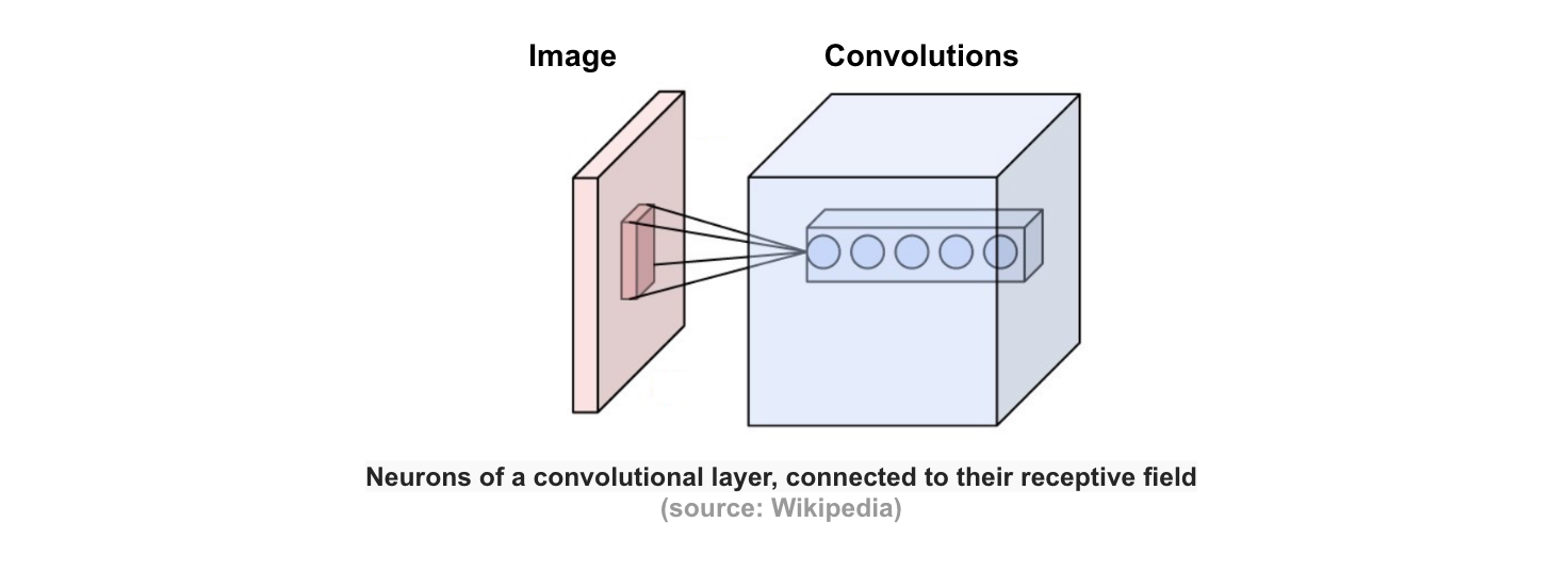
Convolution Layer

This layer consists of a set of learnable filters that we slide over the image spatially, computing dot products between the entries of the filter and the input image. The filters should extend to the full depth of the input image. For example, if we want to apply a filter of size 5x5 to a colored image of size 32x32, then the filter should have depth 3 (5x5x3) to cover all 3 color channels (Red, Green, Blue) of the image. These filters will activate when they see same specific structure in the images.

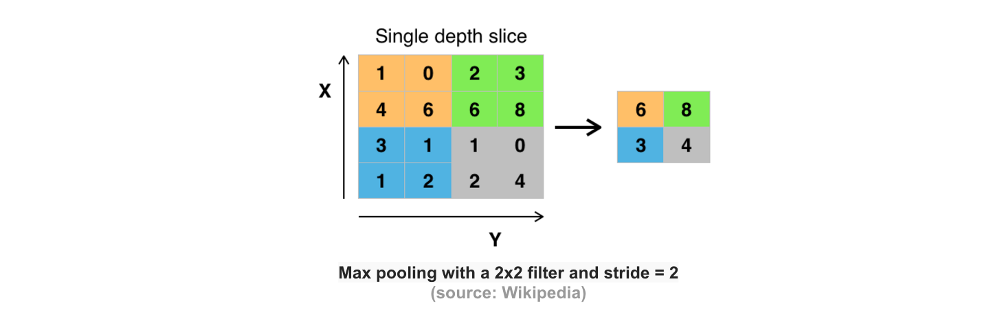
Pooling Layer

Pooling is a form of non-linear down-sampling. The goal of the pooling layer is to progressively reduce the spatial size of the representation to reduce the amount of parameters and computation in the network, and hence to also control overfitting. There are several functions to implement pooling among which max pooling is the most common one. Pooling is often applied with filters of size 2x2 applied with a stride of 2 at every depth slice. A pooling layer of size 2x2 with stride of 2 shrinks the input image to a 1/4 of its original size. [2]

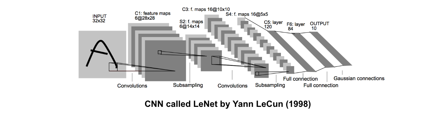
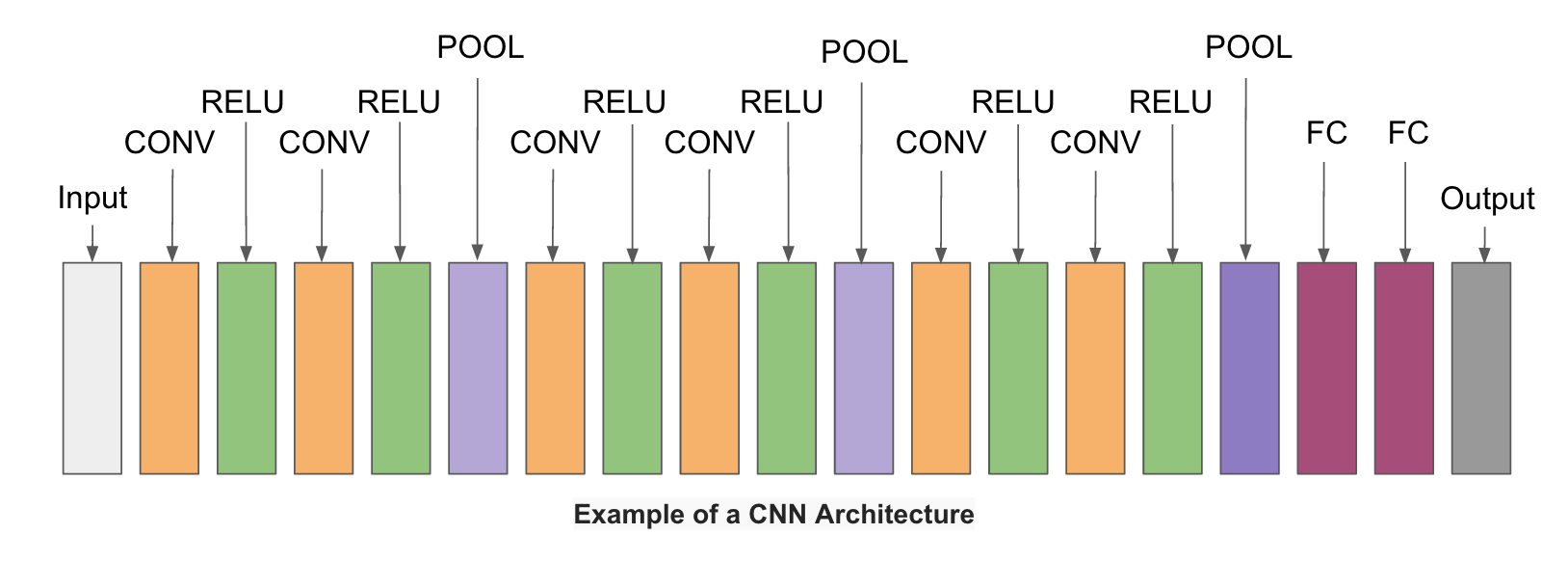
Convolutional Neural Networks Architecture

The simplest architecture of a convolutional neural networks starts with an input layer (images) followed by a sequence of convolutional layers and pooling layers, and ends with fully-connected layers. The convolutional layers are usually followed by one layer of ReLU activation functions.

The convolutional, pooling and ReLU layers act as learnable features extractors, while the fully connected layers acts as a machine learning classifier. Furthermore, the early layers of the network encode generic patterns of the images, while later layers encode the details patterns of the images.

Note that only the convolutional layers and fully-connected layers have weights. These weights are learned in the training phase.

4. Building a Cat/Dog Classifier using a Convolutional Neural Network

In this section, we will implement a cat/dog classifier using a convolutional neural network. We will use a dataset from Kaggle's Dogs vs. Cats competition. To implement the convolutional neural network, we will use a deep learning framework called Caffe and some Python code.

4.1 Getting Dogs & Cats Data

First, we need to download 2 datasets from the competition page: train.zip and test1.zip. The train.zip file contains labeled cats and dogs images that we will use to train the network. The test1.zip file contains unlabeled images that we will classify to either dog or cat using the trained model. We will upload our predictions to Kaggle to get the score of our prediction model.

4.2 Machine Setup

To train convolutional neural networks, we need a machine with a powerful GPU.

In this tutorial, I used one AWS EC2 instance of type g2.2xlarge. This instance has a high-performance NVIDIA GPU with 1,536 CUDA cores and 4GB of video memory, 15GB of RAM and 8 vCPUs. The machine costs $0.65/hour.

If you're not familiar with AWS, this guide will help you set up an AWS EC2 instance.

Please note, that the AMI recommended in the guide is no longer available. I prepared a new AMI (ami-64d31209) with all the necessary software installed. I also created a guide for installing Caffe and Anaconda on an AWS EC2 instance or an Ubuntu machine with GPU.

After setting up an AWS instance, we connect to it and clone the github repository that contains the necessary Python code and Caffe configuration files for the tutorial. From your terminal, execute the following command.

git clone https://github.com/adilmoujahid/deeplearning-cats-dogs-tutorial.git

Next, we create an input folder for storing the training and test images.

cd deeplearning-cats-dogs-tutorial
mkdir input

4.3 Caffe Overview

Caffe is a deep learning framework developed by the Berkeley Vision and Learning Center (BVLC). It is written in C++ and has Python and Matlab bindings.

There are 4 steps in training a CNN using Caffe:

• Step 1 - Data preparation: In this step, we clean the images and store them in a format that can be used by Caffe. We will write a Python script that will handle both image pre-processing and storage.
• Step 2 - Model definition: In this step, we choose a CNN architecture and we define its parameters in a configuration file with extension .prototxt.
• Step 3 - Solver definition: The solver is responsible for model optimization. We define the solver parameters in a configuration file with extension .prototxt.
• Step 4 - Model training: We train the model by executing one Caffe command from the terminal. After training the model, we will get the trained model in a file with extension .caffemodel.

After the training phase, we will use the .caffemodel trained model to make predictions of new unseen data. We will write a Python script to this.

4.4 Data Preparation

We start by copying the train.zip and test1.zip (that we downloaded to our local machine) to the input folder in the AWS instance. We can do this using the scp command from a MAC or linux machine. If you're running Windows, you can use a program such as Winscp. After copying the data, we unzip the files by executing the following commands:

unzip ~/deeplearning-cats-dogs-tutorial/input/train.zip
unzip ~/deeplearning-cats-dogs-tutorial/input/test1.zip
rm ~/deeplearning-cats-dogs-tutorial/input/*.zip

Next, we run create_lmdb.py.

cd ~/deeplearning-cats-dogs-tutorial/code
python create_lmdb.py

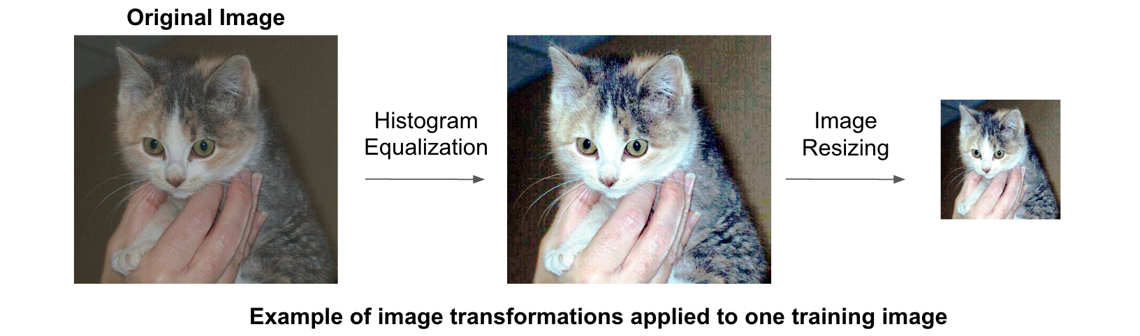
create_lmdb.py script does the following:

• Run histogram equalization on all training images. Histogram equalization is a technique for adjusting the contrast of images.
• Resize all training images to a 227x227 format.
• Divide the training data into 2 sets: One for training (5/6 of images) and the other for validation (1/6 of images). The training set is used to train the model, and the validation set is used to calculate the accuracy of the model.
• Store the training and validation in 2 LMDB databases. train_lmdb for training the model and validation_lmbd for model evaluation.

Below is the explanation of the most important parts of the code.

def transform_img(img, img_width=IMAGE_WIDTH, img_height=IMAGE_HEIGHT):

    #Histogram Equalization
    img[:, :, 0] = cv2.equalizeHist(img[:, :, 0])
    img[:, :, 1] = cv2.equalizeHist(img[:, :, 1])
    img[:, :, 2] = cv2.equalizeHist(img[:, :, 2])

    #Image Resizing
    img = cv2.resize(img, (img_width, img_height), interpolation = cv2.INTER_CUBIC)

    return img

transform_img takes a colored images as input, does the histogram equalization of the 3 color channels and resize the image.

def make_datum(img, label):

    return caffe_pb2.Datum(
        channels=3,
        width=IMAGE_WIDTH,
        height=IMAGE_HEIGHT,
        label=label,
        data=np.rollaxis(img, 2).tostring())

make_datum takes an image and its label and return a Datum object that contains the image and its label.

in_db = lmdb.open(train_lmdb, map_size=int(1e12))
with in_db.begin(write=True) as in_txn:
    for in_idx, img_path in enumerate(train_data):
        if in_idx %  6 == 0:
            continue
        img = cv2.imread(img_path, cv2.IMREAD_COLOR)
        img = transform_img(img, img_width=IMAGE_WIDTH, img_height=IMAGE_HEIGHT)
        if 'cat' in img_path:
            label = 0
        else:
            label = 1
        datum = make_datum(img, label)
        in_txn.put('{:0>5d}'.format(in_idx), datum.SerializeToString())
        print '{:0>5d}'.format(in_idx) + ':' + img_path
in_db.close()

The code above takes 5/6 of the training images, transforms and stores them in train_lmdb. The code for storing validation data follows the same structure.

Generating the mean image of training data

We execute the command below to generate the mean image of training data. We will substract the mean image from each input image to ensure every feature pixel has zero mean. This is a common preprocessing step in supervised machine learning.

/home/ubuntu/caffe/build/tools/compute_image_mean -backend=lmdb /home/ubuntu/deeplearning-cats-dogs-tutorial/input/train_lmdb /home/ubuntu/deeplearning-cats-dogs-tutorial/input/mean.binaryproto

4.4 Model Definition

After deciding on the CNN architecture, we need to define its parameters in a .prototxt train_val file. Caffe comes with a few popular CNN models such as Alexnet and GoogleNet. In this tutorial, we will use the bvlc_reference_caffenet model which is a replication of AlexNet with a few modifications. Below is a copy of the train_val file that we call caffenet_train_val_1.prototxt. If you clone the tutorial git repository as explained above, you should have the same file under deeplearning-cats-dogs-tutorial/caffe_models/caffe_model_1/.

We need to make the modifications below to the original bvlc_reference_caffenet prototxt file:

• Change the path for input data and mean image: Lines 24, 40 and 51.
• Change the number of outputs from 1000 to 2: Line 373. The original bvlc_reference_caffenet was designed for a classification problem with 1000 classes.

We can print the model architecture by executing the command below. The model architecture image will be stored under deeplearning-cats-dogs-tutorial/caffe_models/caffe_model_1/caffe_model_1.png

python /home/ubuntu/caffe/python/draw_net.py /home/ubuntu/deeplearning-cats-dogs-tutorial/caffe_models/caffe_model_1/caffenet_train_val_1.prototxt /home/ubuntu/deeplearning-cats-dogs-tutorial/caffe_models/caffe_model_1/caffe_model_1.png

4.5 Solver Definition

The solver is responsible for model optimization. We define the solver's parameters in a .prototxt file. You can find our solver under deeplearning-cats-dogs-tutorial/caffe_models/caffe_model_1/ with name solver_1.prototxt. Below is a copy of the same.

This solver computes the accuracy of the model using the validation set every 1000 iterations. The optimization process will run for a maximum of 40000 iterations and will take a snapshot of the trained model every 5000 iterations.

base_lr, lr_policy, gamma, momentum and weight_decay are hyperparameters that we need to tune to get a good convergence of the model.

I chose lr_policy: "step" with stepsize: 2500, base_lr: 0.001 and gamma: 0.1. In this configuration, we will start with a learning rate of 0.001, and we will drop the learning rate by a factor of ten every 2500 iterations.

There are different strategies for the optimization process. For a detailed explanation, I recommend Caffe's solver documentation.

4.6 Model Training

After defining the model and the solver, we can start training the model by executing the command below:

/home/ubuntu/caffe/build/tools/caffe train --solver /home/ubuntu/deeplearning-cats-dogs-tutorial/caffe_models/caffe_model_1/solver_1.prototxt 2>&1 | tee /home/ubuntu/deeplearning-cats-dogs-tutorial/caffe_models/caffe_model_1/model_1_train.log

The training logs will be stored under deeplearning-cats-dogs-tutorial/caffe_models/caffe_model_1/model_1_train.log.

During the training process, we need to monitor the loss and the model accuracy. We can stop the process at anytime by pressing Ctrl+c. Caffe will take a snapshot of the trained model every 5000 iterations, and store them under caffe_model_1 folder.

The snapshots have .caffemodel extension. For example, 10000 iterations snapshot will be called: caffe_model_1_iter_10000.caffemodel.

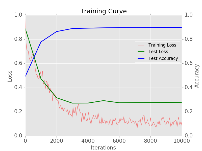
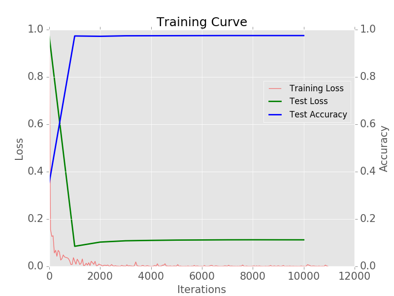
Plotting the learning curve

A learning curve is a plot of the training and test losses as a function of the number of iterations. These plots are very useful to visualize the train/validation losses and validation accuracy.

We can see from the learning curve that the model achieved a validation accuracy of 90%, and it stopped improving after 3000 iterations.

python /home/ubuntu/deeplearning-cats-dogs-tutorial/caffe_models/code/plot_learning_curve.py /home/ubuntu/deeplearning-cats-dogs-tutorial/caffe_models/caffe_models/caffe_model_1/model_1_train.log /home/ubuntu/deeplearning-cats-dogs-tutorial/caffe_models/caffe_models/caffe_model_1/caffe_model_1_learning_curve.png

4.7 Prediction on New Data

Now that we have a trained model, we can use it to make predictions on new unseen data (images from test1). The Python code for making the predictions is make_predictions_1.py and it's stored under deeplearning-cats-dogs-tutorial/code. The code needs 4 files to run:

• Test images: We will use test1 images.
• Mean image: The mean image that we computed in section 4.4.
• Model architecture file: We'll call this file caffenet_deploy_1.prototxt. It's stored under deeplearning-cats-dogs-tutorial/caffe_models/caffe_model_1. It's structured in a similar way to caffenet_train_val_1.prototxt, but with a few modifications. We need to delete the data layers, add an input layer and change the last layer type from SoftmaxWithLoss to Softmax.
• Trained model weights: This is the file that we computed in the training phase. We will use caffe_model_1_iter_10000.caffemodel.

To run the Python code, we need to execute the command below. The predictions will be stored under deeplearning-cats-dogs-tutorial/caffe_models/caffe_model_1/submission_model_1.csv.

cd /home/ubuntu/deeplearning-cats-dogs-tutorial/code
python make_predictions_1.py

Below is the explanation of the most important parts in the code.

#Read mean image
mean_blob = caffe_pb2.BlobProto()
with open('/home/ubuntu/deeplearning-cats-dogs-tutorial/input/mean.binaryproto') as f:
    mean_blob.ParseFromString(f.read())
mean_array = np.asarray(mean_blob.data, dtype=np.float32).reshape(
    (mean_blob.channels, mean_blob.height, mean_blob.width))


#Read model architecture and trained model's weights
net = caffe.Net('/home/ubuntu/deeplearning-cats-dogs-tutorial/caffe_models/caffe_model_1/caffenet_deploy_1.prototxt',
                '/home/ubuntu/deeplearning-cats-dogs-tutorial/caffe_models/caffe_model_1/caffe_model_1_iter_10000.caffemodel',
                caffe.TEST)

#Define image transformers
transformer = caffe.io.Transformer({'data': net.blobs['data'].data.shape})
transformer.set_mean('data', mean_array)
transformer.set_transpose('data', (2,0,1))

The code above stores the mean image under mean_array, defines a model called net by reading the deploy file and the trained model, and defines the transformations that we need to apply to the test images.

img = cv2.imread(img_path, cv2.IMREAD_COLOR)
img = transform_img(img, img_width=IMAGE_WIDTH, img_height=IMAGE_HEIGHT)

net.blobs['data'].data[...] = transformer.preprocess('data', img)
out = net.forward()
pred_probas = out['prob']
print pred_probas.argmax()

The code above read an image, apply similar image processing steps to training phase, calculates each class' probability and prints the class with the largest probability (0 for cats, and 1 for dogs).

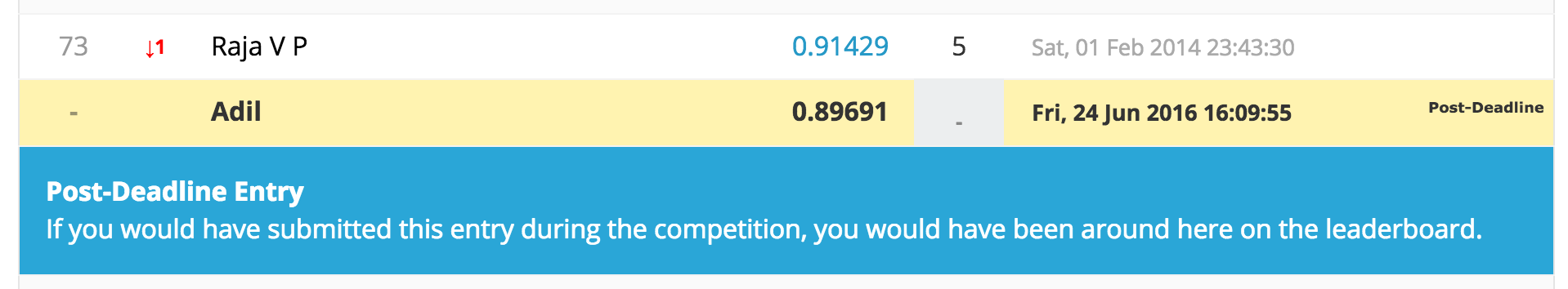
After submitting the predicitions to Kaggle, it give an accuracy of 0.89691.

5. Building a Cat/Dog Classifier using Transfer Learning

In this section, we will use a very practical and powerful technique called transfer learning for building our cat/dog classifier.

5.1 What is Transfer Learning?

Convolutional neural networks require large datasets and a lot of computional time to train. Some networks could take up to 2-3 weeks across multiple GPUs to train. Transfer learning is a very useful technique that tries to address both problems. Instead of training the network from scratch, transfer learning utilizes a trained model on a different dataset, and adapts it to the problem that we're trying to solve.

There are 2 strategies for transfer learning:

• Utilize the trained model as a fixed feature extractor: In this strategy, we remove the last fully connected layer from the trained model, we freeze the weights of the remaining layers, and we train a machine learning classifier on the output of the remaining layers.
• Fine-tune the trained model: In this strategy, we fine tune the trained model on the new dataset by continuing the backpropagation. We can either fine-tune the whole network or freeze some of its layers.

For a detailed explanation of transfer learning, I recommend reading these notes.

5.2 Training the Cat/Dog Classifier using Transfer Learning

Caffe comes with a repository that is used by researchers and machine learning practitioners to share their trained models. This library is called Model Zoo.

We will utilize the trained bvlc_reference_caffenet as a starting point of building our cat/dog classifier using transfer learning. This model was trained on the ImageNet dataset which contains millions of images across 1000 categories.

We will use the fine-tuning strategy for training our model.

Download trained bvlc_reference_caffenet model

We can download the trained model by executing the command below.

cd /home/ubuntu/caffe/models/bvlc_reference_caffenet
wget http://dl.caffe.berkeleyvision.org/bvlc_reference_caffenet.caffemodel

Model Definition

The model and solver configuration files are stored under deeplearning-cats-dogs-tutorial/caffe_models/caffe_model_2. We need to make the following change to the original bvlc_reference_caffenet model configuration file.

• Change the path for input data and mean image: Lines 24, 40 and 51.
• Change the name of the last fully connected layer from fc8 to fc8-cats-dogs. Lines 360, 363, 387 and 397.
• Change the number of outputs from 1000 to 2: Line 373. The original bvlc_reference_caffenet was designed for a classification problem with 1000 classes.

Note that if we keep a layer's name unchanged and we pass the trained model's weights to Caffe, it will pick its weights from the trained model. If we want to freeze a layer, we need to setup its lr_mult parameter to 0.

Solver Definition

We will use a similar solver to the one used in section 4.5.

Model Training with Transfer Learning

After defining the model and the solver, we can start training the model by executing the command below. Note that we can pass the trained model's weights by using the argument --weights.

/home/ubuntu/caffe/build/tools/caffe train --solver=/home/ubuntu/deeplearning-cats-dogs-tutorial/caffe_models/caffe_model_2/solver_2.prototxt --weights /home/ubuntu/caffe/models/bvlc_reference_caffenet/bvlc_reference_caffenet.caffemodel 2>&1 | tee /home/ubuntu/deeplearning-cats-dogs-tutorial/caffe_models/caffe_model_2/model_2_train.log

Plotting the Learning Curve

Similarly to the previous section, we can plot the learning curve by executing the command below. We can see from the learning curve that the model achieved an accuracy of ~97% after 1000 iterations only. This shows the power of transfer learning. We were able to get a higher accuracy with a smaller number of iterations.

python /home/ubuntu/deeplearning-cats-dogs-tutorial/code/plot_learning_curve.py /home/ubuntu/deeplearning-cats-dogs-tutorial/caffe_models/caffe_model_2/model_2_train.log /home/ubuntu/deeplearning-cats-dogs-tutorial/caffe_models/caffe_model_2/caffe_model_2_learning_curve.png

Prediction on New Data

Similary to section 4.7, we will generate predictions on the test data and upload the results to Kaggle to get the model accuracy. The code for making the predicitions is under deeplearning-cats-dogs-tutorial/code/make_predictions_2.py.

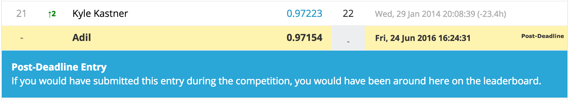
The model got an accuracy of 0.97154 which is better than the model that we trained from scratch.

Conclusion

In this blog post, we covered core concepts of deep learning and convolutional neural networks. We also learned how to build convolutional neural networks using Caffe and Python from scratch and using transfer learning. If you want to learn more about this topic, I highly recommend Stanford's "Convolutional Neural Networks for Visual Recognition" course.

References

1. CS231n - Neural Networks Part 1: Setting up the Architecture
2. Wikipedia - Convolutional Neural Network
3. CS231n - Transfer Learning Notes
4. A Step by Step Backpropagation Example
5. CS231n Convolutional Neural Networks for Visual Recognition