Adil Moujahid

Follow @AdilMouja

Published

Sun 12 April 2020

←Home

Analyzing the Impact of Coronavirus on the Stock Market using Python, Google Sheets and Google Finance

// tags python pandas

Since its emergence in Asia late 2019, the coronavirus COVID-19 pandemic has been devastating. The virus spread to most countries causing severe respiratory infections and many human casualties. The virus also put half of the world population in lockdown which resulted in a slowdown of the world economy and a fall in stock prices.

The goal of this tutorial is to introduce the steps for collecting and analyzing stock data in the context of the coronavirus pandemic. To do this, we will use Python, Google Sheets and Google Finance.

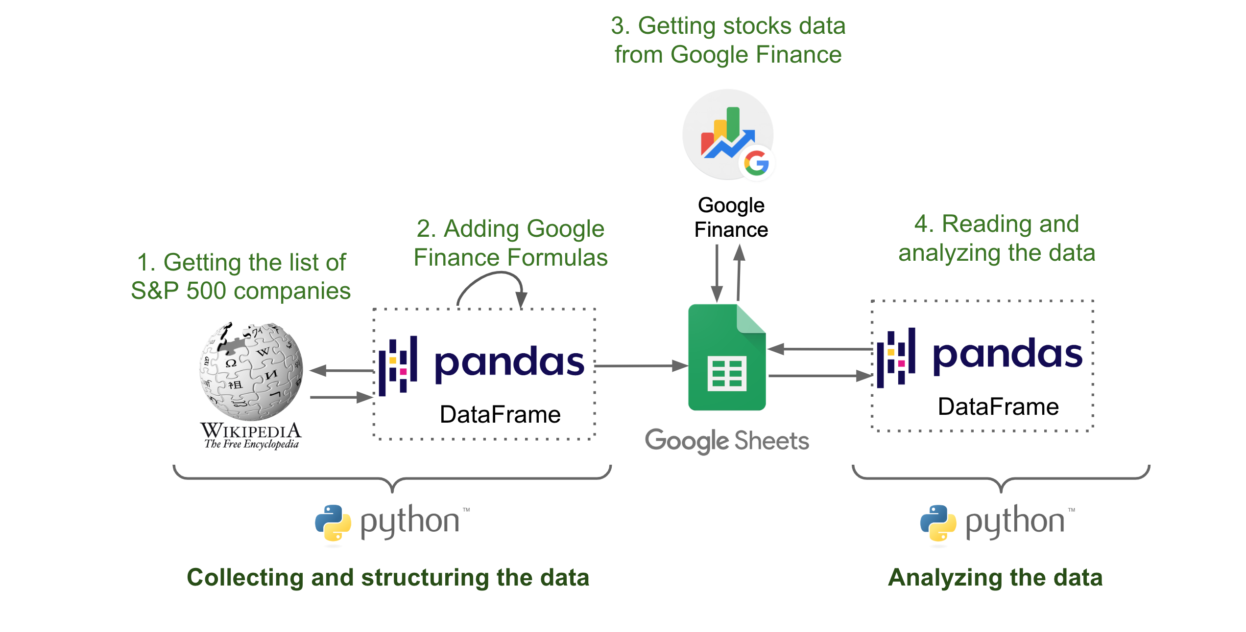
In section 2 of the the tutorial, we will see how to configure Google Sheets in order to be able to interact with them using Python. In section 3, we will see how to collect stocks data using Google Finance and how to store this data in Google Sheets using Python. In section 4, we will see how to read the data from Google Sheets and analyze it using Python and Pandas.

The source code for this tutorial can be found in this github repository.

1. The Case Study

In this tutorial, we will focus on the S&P 500 companies. We will start by collecting the following data :

• Stock prices in 3 different dates (January 1st, March 23rd and April 9th)
• Number of outstanding shares for each company
• Industry/Sector where the companies operate (following the GICS classification)

After collecting and structuring the data, we will use Python and Pandas library to analyse the data.

2. Technical Setup

We will be using the following services and libraries to collect and analyze the data:

• Wikipedia: We will use this wikipedia page to get the list of S&P 500 companies.
• Google Finance: Google Finance is a website focusing on business news and financial information hosted by Google [1]. Google Finance doesn't have an API that we can use directly in Python, but it can be accessed from Google Sheets using a formula called GOOGLEFINANCE. We will use Python to write down the GOOGLEFINANCE formulas.
• Goole Sheets: We will use Google Sheets as a backend to store stocks data. In order to interact with Google Sheets directly from Python, we need 3 libaries: Google Auth, gspread and gspread-pandas. We also need to configure Google Sheets to be able to access the spreadsheets using Python.
• Python and Jupyter notebooks and Pandas: We will be using Python, Jupyter notebooks and Pandas to collect, store and analyze the data.

2.1. Google Sheets Configuration in GCP

In order to access Google Sheets from Python, we need a private key from Google Cloud Platfrom (GCP) that we can obtain using the following steps.

• Step 1: Go to Google Cloud platform, log in using your google account and click on Console.

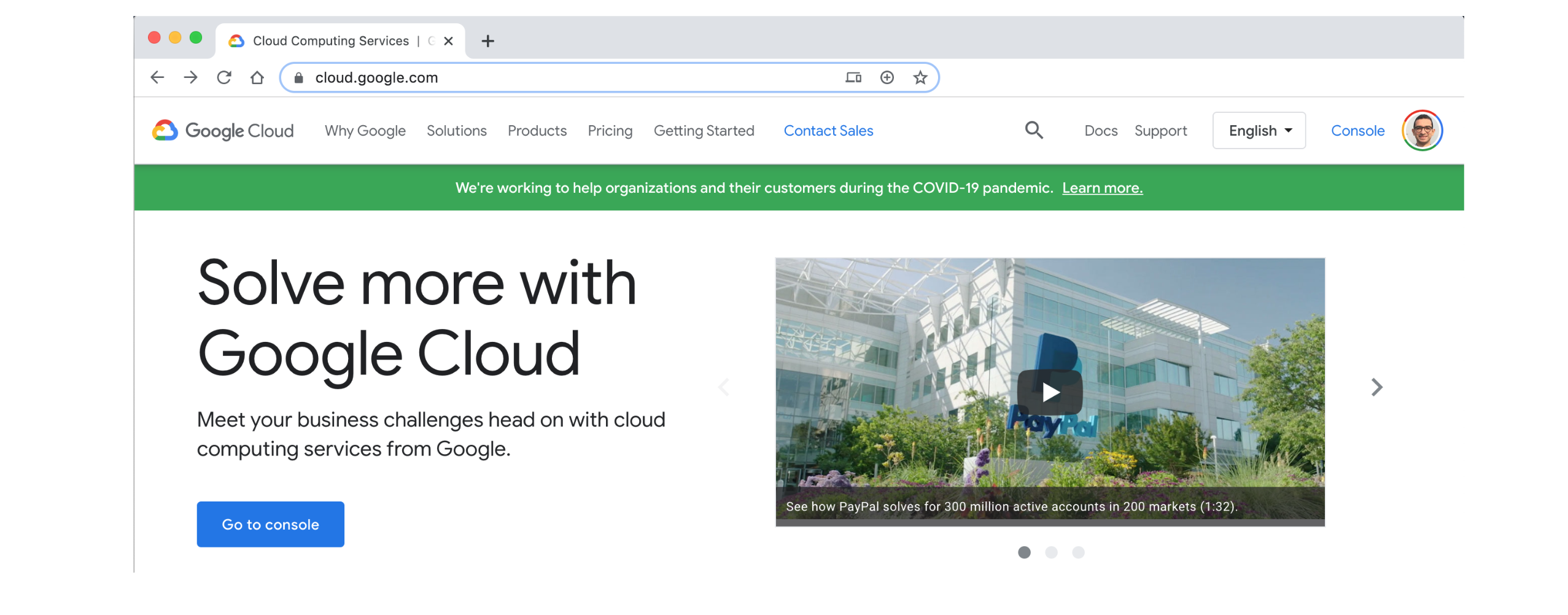
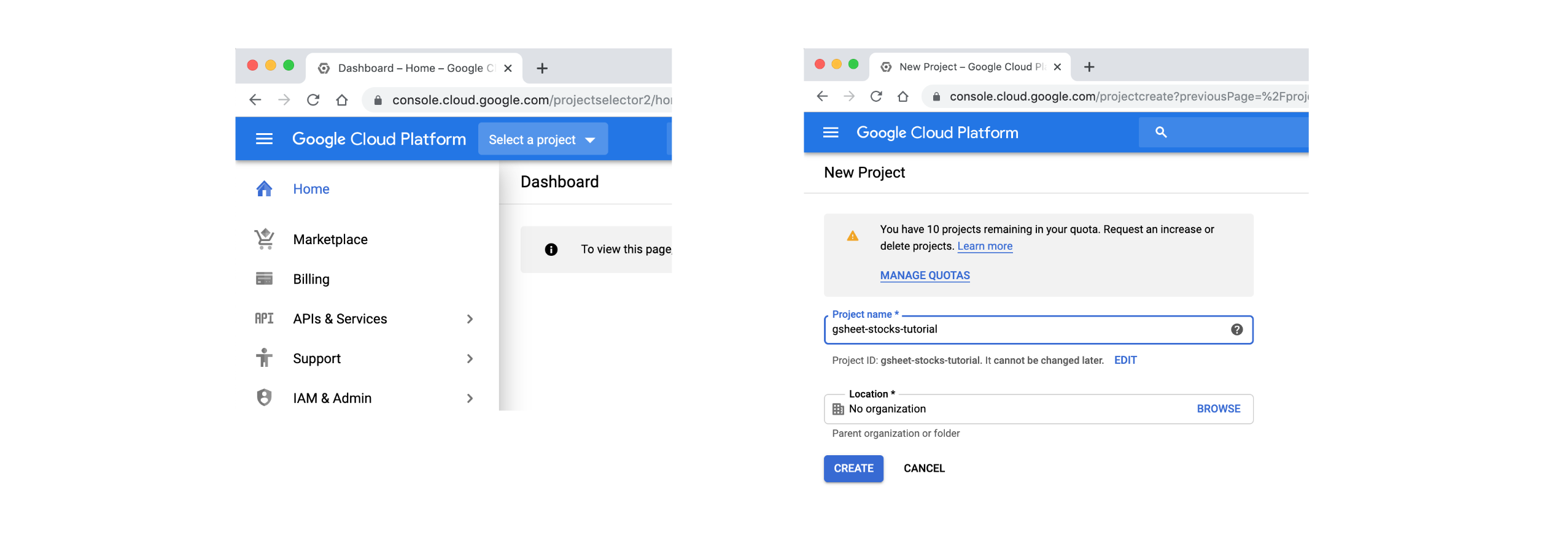
• Step 2: Click on Select a project > NEW PROJECT, enter the project name and click on CREATE

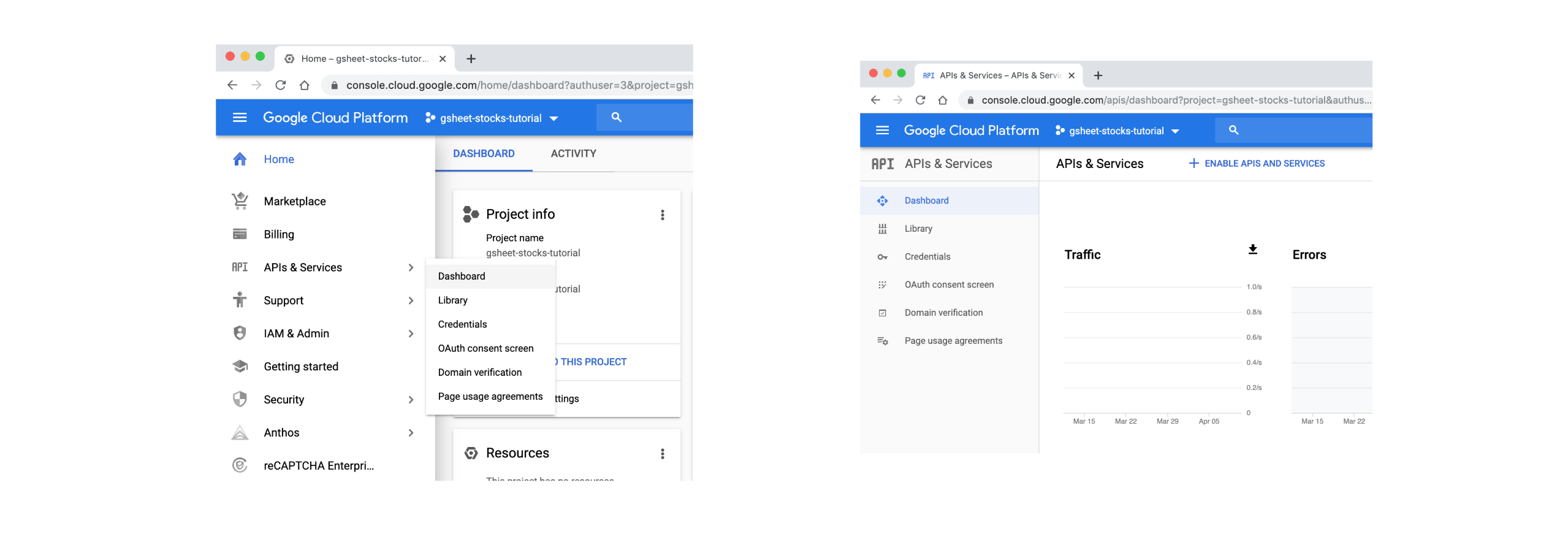
• Step 3: Click on APIs & Services > Dashboard > ENABLE APIS AND SEVICES.

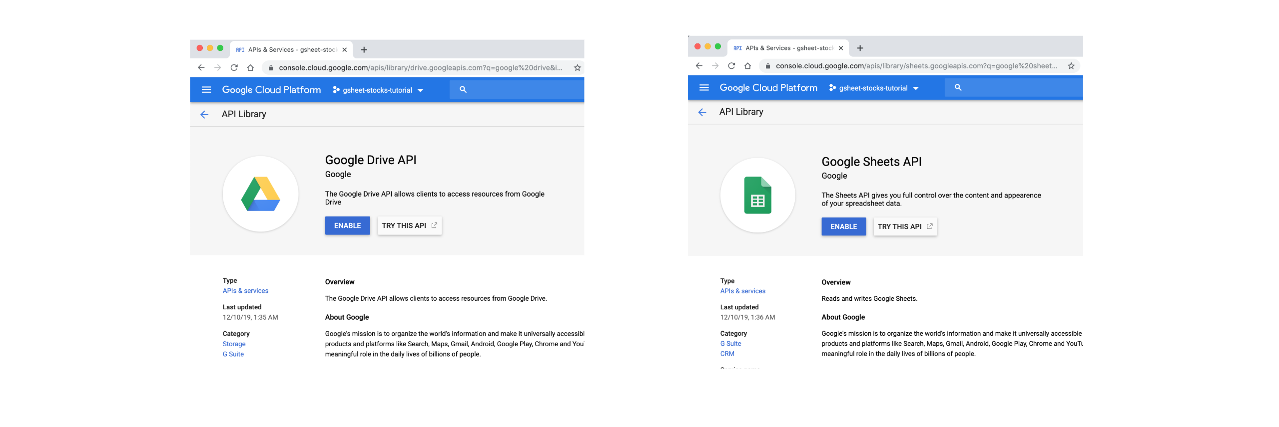
• Step 4: Search for both Google Drive API and Google Sheets API and click on ENABLE

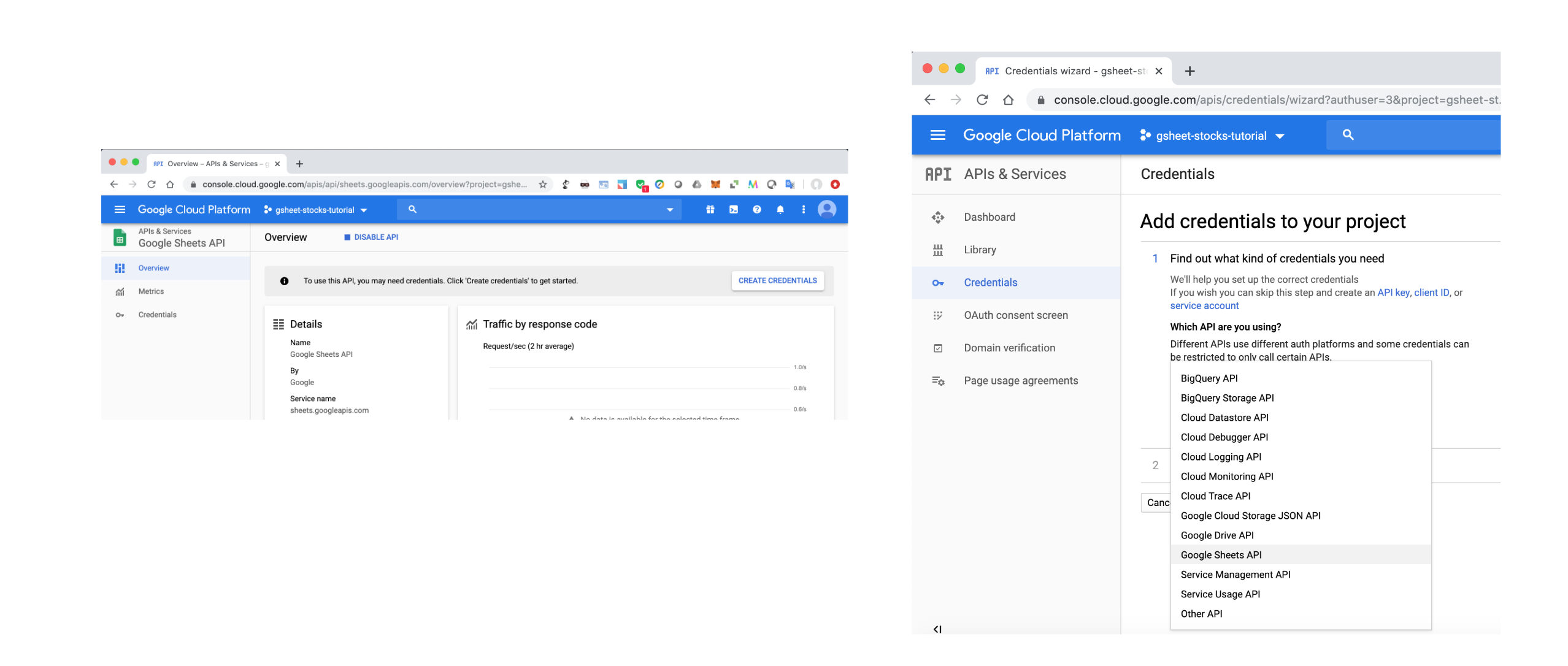
• Step 5: Inside the Google Sheets API page, click on MANAGE, CREATE CREDENTIALS and select Google Sheets API.

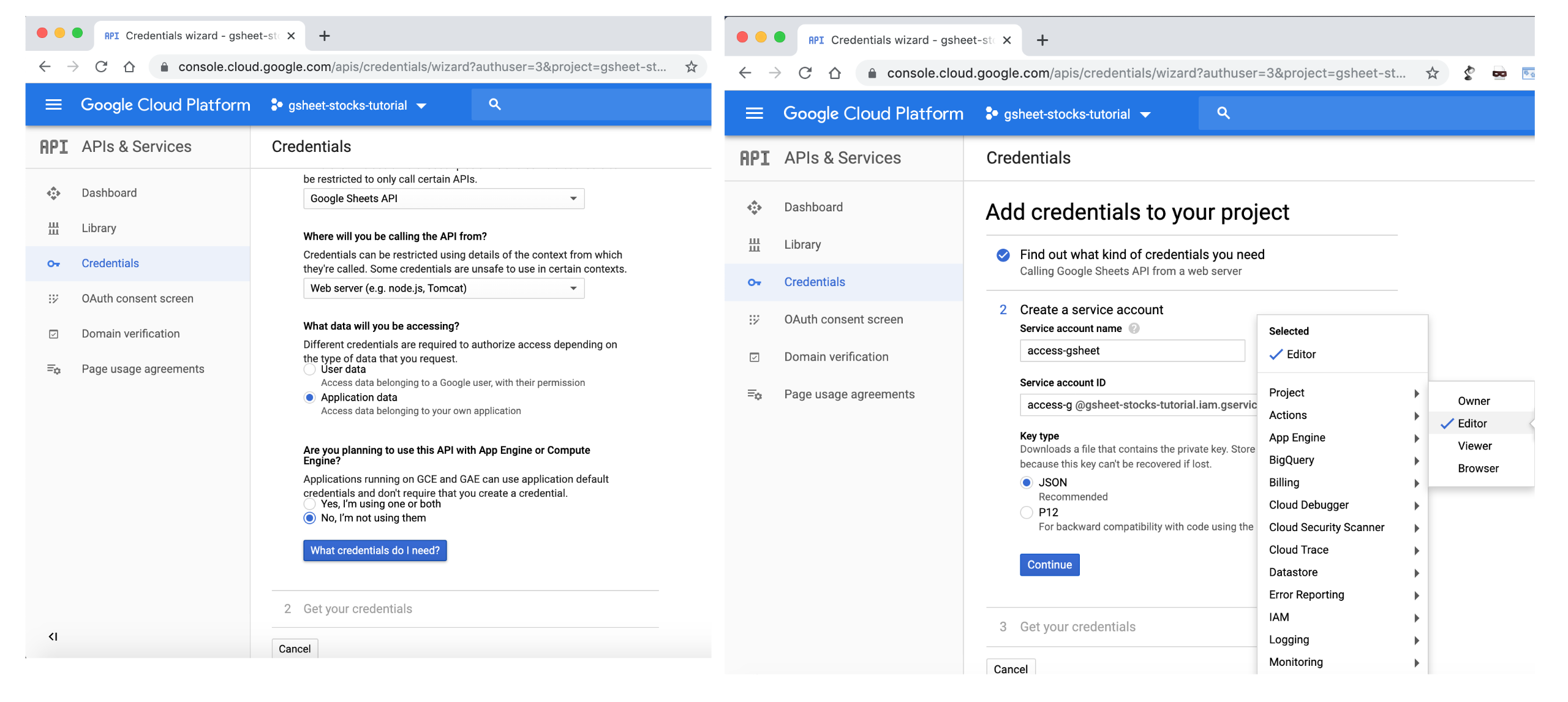
• Step 6: Choose Web sever, Application data and JSON type for the API key. Click Continue to download your private key in JSON format.

• Step 7: Once you download the JSON file, save in the same folder as your Jupyter notebook and copy the client_email information.

2.2. Google Sheets Configuration

As a last step, we need to create a new Google sheet and share it with the client_email that we created in the previous step. Open Google Drive, create a new Google Sheet, change its name to "stocks-data". Click on Share button, enter the client_email and click Send.

3. Collecting and Storing Stocks Data

Now that we have our google Sheets configured, we can start using Python and Jupyter Notebook to collect the data. We start by importing the different libraries that we need.

%matplotlib inline

import pandas as pd
import gspread
from google.oauth2.service_account import Credentials
from gspread_pandas import Spread, Client

import seaborn as sns 
import matplotlib.pyplot as plt

plt.style.use('fivethirtyeight')

Getting the list of S&P 500 companies from Wikipedia

As a first step in the data collection effort, we need to get the list of S&P 500 companies. To do this, we will use the following Wikipedia Page: https://en.wikipedia.org/wiki/List_of_S%26P_500_companies

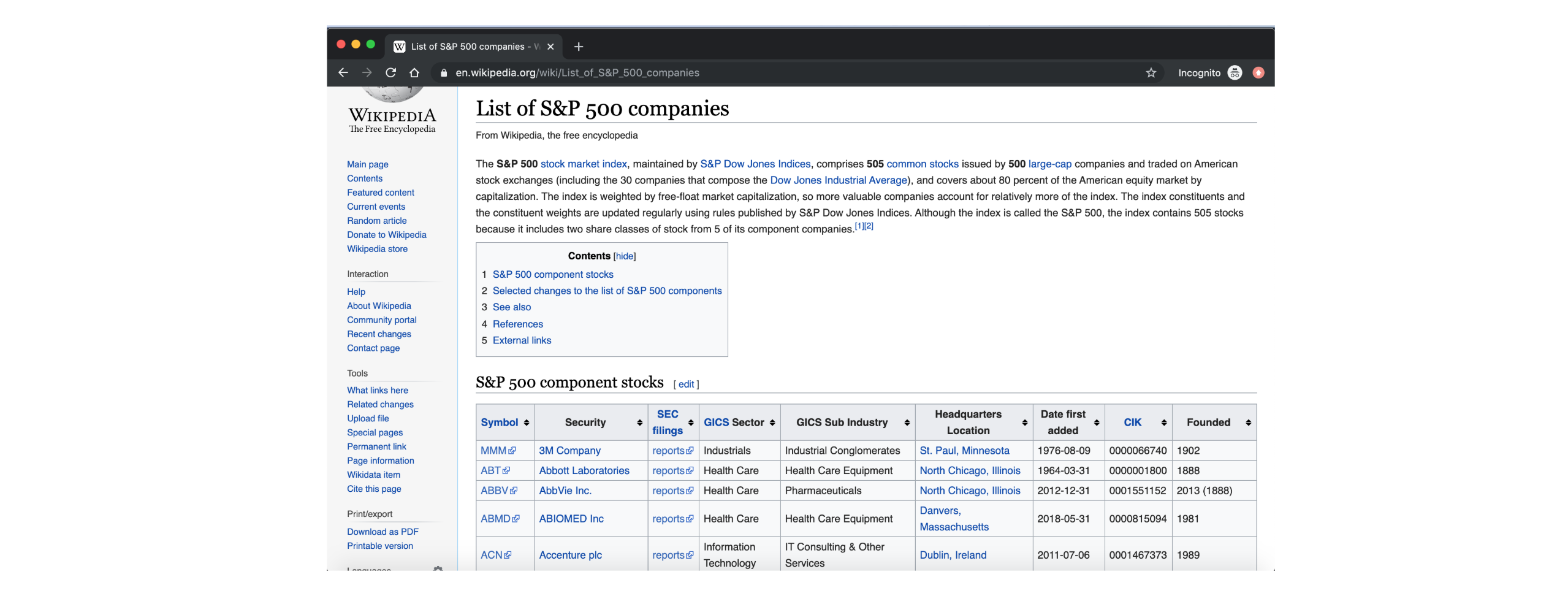
Fortunatey, we can use Pandas to read the page, extract the table with S&P 500 companies and store them into a Pandas Dataframe.

url = 'https://en.wikipedia.org/wiki/List_of_S%26P_500_companies'

stocks_df = pd.read_html(url, header=0)[0]

stocks_df.head()

	Symbol	Security	SEC filings	GICS Sector	GICS Sub Industry	Headquarters Location	Date first added	CIK	Founded
0	MMM	3M Company	reports	Industrials	Industrial Conglomerates	St. Paul, Minnesota	1976-08-09	66740	1902
1	ABT	Abbott Laboratories	reports	Health Care	Health Care Equipment	North Chicago, Illinois	1964-03-31	1800	1888
2	ABBV	AbbVie Inc.	reports	Health Care	Pharmaceuticals	North Chicago, Illinois	2012-12-31	1551152	2013 (1888)
3	ABMD	ABIOMED Inc	reports	Health Care	Health Care Equipment	Danvers, Massachusetts	2018-05-31	815094	1981
4	ACN	Accenture plc	reports	Information Technology	IT Consulting & Other Services	Dublin, Ireland	2011-07-06	1467373	1989

The most important data that we need is:

• Symbol: Stock Symbol
• Security: Name of the company
• GICS Sector: Sector where the company operates following the Global Industry Classification Standard (GICS).
• GICS Sub Industry: Sub industry where the company operates following the Global Industry Classification Standard (GICS).

We can start looking at some statistics. For example the number of companies in the list.

#Number of companis
len(stocks_df)

505

We got 505 companies in our list, and not 500... This is because some companies have a dual-class stock structure and are listed more than once in the list. We can get the list of these companies by searching for the word "Class" in their security name.

stocks_df[stocks_df['Security'].str.contains("Class")]

	Symbol	Security	SEC filings	GICS Sector	GICS Sub Industry	Headquarters Location	Date first added	CIK	Founded
24	GOOGL	Alphabet Inc Class A	reports	Communication Services	Interactive Media & Services	Mountain View, California	2014-04-03	1652044	1998
25	GOOG	Alphabet Inc Class C	reports	Communication Services	Interactive Media & Services	Mountain View, California	2006-04-03	1652044	1998
148	DISCA	Discovery Inc. Class A	reports	Communication Services	Broadcasting	Silver Spring, Maryland	2010-03-01	1437107	NaN
149	DISCK	Discovery Inc. Class C	reports	Communication Services	Broadcasting	Silver Spring, Maryland	2014-08-07	1437107	NaN
203	FOXA	Fox Corporation Class A	reports	Communication Services	Movies & Entertainment	New York, New York	2013-07-01	1308161	NaN
204	FOX	Fox Corporation Class B	reports	Communication Services	Movies & Entertainment	New York, New York	2015-09-18	1308161	NaN
340	NWSA	News Corp. Class A	reports	Communication Services	Publishing	New York, New York	2013-08-01	1564708	NaN
341	NWS	News Corp. Class B	reports	Communication Services	Publishing	New York, New York	2015-09-18	1564708	NaN
457	UAA	Under Armour Class A	reports	Consumer Discretionary	Apparel, Accessories & Luxury Goods	Baltimore, Maryland	2014-05-01	1336917	NaN
458	UA	Under Armour Class C	reports	Consumer Discretionary	Apparel, Accessories & Luxury Goods	Baltimore, Maryland	2016-04-08	1336917	NaN

We got 10 companies with dual-class structure in the list. If we take that into consideration, we can see that we have 500 unique companies in the list.

We can also check the number of companies by sector and sub industry.

stocks_df['GICS Sector'].value_counts()

Industrials               71
Information Technology    71
Financials                66
Consumer Discretionary    64
Health Care               60
Consumer Staples          33
Real Estate               31
Utilities                 28
Materials                 28
Energy                    27
Communication Services    26
Name: GICS Sector, dtype: int64

stocks_df['GICS Sub Industry'].value_counts()

Health Care Equipment       19
Electric Utilities          13
Semiconductors              13
Industrial Machinery        13
Packaged Foods & Meats      12
                            ..
Real Estate Services         1
Motorcycle Manufacturers     1
Multi-Sector Holdings        1
Hotel & Resort REITs         1
Drug Retail                  1
Name: GICS Sub Industry, Length: 128, dtype: int64

Adding stocks data from Google Finance

Now that we have the list of S&P 500 companies, we can add to our DataFrame Google Sheets formulas that will fetch from Google Finance stock prices and the number of outstanding shares for each company. Note that, these formulas will be executed once we save the Pandas DataFrame in our Google Sheet.

You can find the documentation of GOOGLEFINANCE formulas here: https://support.google.com/docs/answer/3093281

We start by adding stock prices in 3 different dates: January 1st, March 23rd and April 9th.

• January 1st, 2020 is the first date of the year. We want to have this price in order to calculate the price drop since the beggining of 2020.
• March 23rd, 2020 is the date when the S&P 500 reached the bottom in 2020.
• April 9th, 2020 is the last date when the stock market was open (at the time of writing this blog post)

stocks_df["Price_1_1"] = stocks_df["Symbol"].apply(lambda x: '=INDEX(GOOGLEFINANCE("' + x + '","price", "1/1/2020"),2,2)')
stocks_df["Price_3_23"] = stocks_df["Symbol"].apply(lambda x: '=INDEX(GOOGLEFINANCE("' + x + '","price", "3/23/2020"),2,2)')
stocks_df["Price_4_9"] = stocks_df["Symbol"].apply(lambda x: '=INDEX(GOOGLEFINANCE("' + x + '","price", "4/9/2020"),2,2)')

Next, we add the formula to calculate the number of outstanding shares for each company. We can use this data with the stock prices to calculate the market cap of companies at the 3 different dates.

stocks_df["Shares"] = stocks_df["Symbol"].apply(lambda x: '=GOOGLEFINANCE("' + x + '","shares")')

Storing the DataFrame to Google Sheet

We start by creating a variable that contains our credentials that we got from Google Cloud Plaltform.

scope = ['https://spreadsheets.google.com/feeds',
         'https://www.googleapis.com/auth/drive']

credentials = Credentials.from_service_account_file('./gsheet-stocks.json', scopes=scope)

Next, we read the empty google sheet in a variable that we call spread.

client = Client(scope=scope, creds=credentials)
spread = Spread("stocks_analysis", client=client)

We define the list of variables that we want to keep.

cols_to_keep = ["Symbol", "Security", "GICS Sector", "GICS Sub Industry", 
                "Price_1_1", "Price_3_23", "Price_4_9", "Shares"]

The last step is to save the DataFrame to Google Sheets.

spread.df_to_sheet(stocks_df[cols_to_keep])

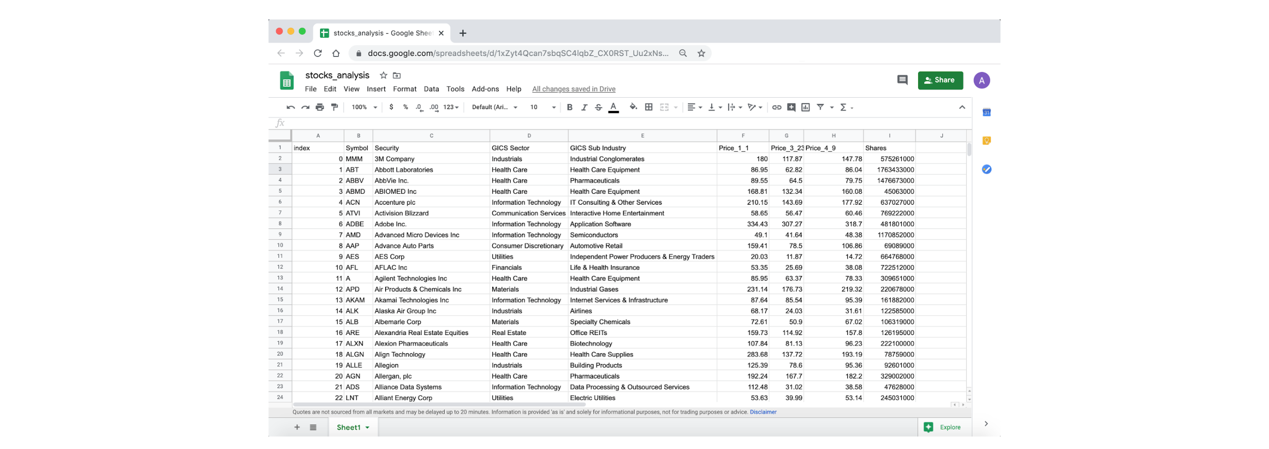
If we go to Google Sheets, we can see that the data is correctly stored.

4. Analyzing the Data

4.1. Reading the data

We start by reading the data from Google Sheets into a new DataFrame.

stocks_df = spread.sheet_to_df()

stocks_df.head()

	Symbol	Security	GICS Sector	GICS Sub Industry	Price_1_1	Price_3_23	Price_4_9	Shares
index
0	MMM	3M Company	Industrials	Industrial Conglomerates	180	117.87	147.78	575261000
1	ABT	Abbott Laboratories	Health Care	Health Care Equipment	86.95	62.82	86.04	1763433000
2	ABBV	AbbVie Inc.	Health Care	Pharmaceuticals	89.55	64.5	79.75	1476673000
3	ABMD	ABIOMED Inc	Health Care	Health Care Equipment	168.81	132.34	160.08	45063000
4	ACN	Accenture plc	Information Technology	IT Consulting & Other Services	210.15	143.69	177.92	637027000

we can see that the DataFrame contains real values for stocks prices and number of shares (and not Google Sheets formulas).

We need to change the data type of stock prices and number of outstanding shares from string to numeric.

stocks_df[["Price_1_1", "Price_3_23", "Price_4_9", "Shares"]] = \
stocks_df[["Price_1_1", "Price_3_23", "Price_4_9", "Shares"]].apply(pd.to_numeric)

4.2. Adding Market Cap data and percentage change of stock prices

Adding Market Cap Data

Next, we will add the market cap in the 3 different dates.

stocks_df["Marketcap_1_1"] = stocks_df["Price_1_1"] * stocks_df["Shares"]
stocks_df["Marketcap_3_23"] = stocks_df["Price_3_23"] * stocks_df["Shares"]
stocks_df["Marketcap_4_9"] = stocks_df["Price_4_9"] * stocks_df["Shares"]

Adding percentage change of stock prices

# Percentage Change from January 1st to March 23rd 
stocks_df["PercentageChange_3_23_1_1"] = (stocks_df["Price_3_23"] - stocks_df["Price_1_1"]) / stocks_df["Price_1_1"]*100
# Percentage Change from March 23rd to April 9th
stocks_df["PercentageChange_4_9_3_23"] = (stocks_df["Price_4_9"] - stocks_df["Price_3_23"]) / stocks_df["Price_3_23"]*100
# # Percentage Change from January 1st to April 9th
stocks_df["PercentageChange_4_9_1_1"] = (stocks_df["Price_4_9"] - stocks_df["Price_1_1"]) / stocks_df["Price_1_1"]*100

4.3. Analyzing the data

Change in the total market cap of the S&P 500

sum(stocks_df["Marketcap_3_23"] - stocks_df["Marketcap_1_1"]) / 10**9

-8713.69057696208

sum(stocks_df["Marketcap_4_9"] - stocks_df["Marketcap_3_23"]) / 10**9

4668.79088967648

sum(stocks_df["Marketcap_4_9"] - stocks_df["Marketcap_1_1"]) / 10**9

-4044.8996872855996

The S&P 500 lost 8.7 trillion USD from January 1st to March 23rd, but it got back 4.6 trillion from March 23rd to April 9th.

Change in the total market cap by sector

(stocks_df.groupby("GICS Sector").sum()["Marketcap_3_23"] - stocks_df.groupby("GICS Sector").sum()["Marketcap_1_1"]).sort_values() / 10**9

GICS Sector
Information Technology   -1592.206753
Financials               -1518.712229
Industrials              -1087.991664
Health Care              -1031.715099
Consumer Discretionary    -793.938427
Communication Services    -734.977458
Energy                    -710.786571
Consumer Staples          -450.846959
Real Estate               -265.205780
Materials                 -264.696109
Utilities                 -262.613530
dtype: float64

At the 2020 bottom of the S&P 500 (March 23rd), the Information Technology and Financials sectors had the largest drop in total market cap (compared to January 1st) with 1.592 trillion and 1.518 trillion respectively.

(stocks_df.groupby("GICS Sector").sum()["Marketcap_4_9"] - stocks_df.groupby("GICS Sector").sum()["Marketcap_1_1"]).sort_values() / 10**9

GICS Sector
Financials               -870.187706
Industrials              -691.882829
Information Technology   -559.803630
Energy                   -510.373229
Communication Services   -401.445690
Consumer Discretionary   -397.755029
Health Care              -269.510749
Consumer Staples         -138.054799
Materials                -110.571043
Real Estate               -55.584791
Utilities                 -39.730193
dtype: float64

As of April 9th, we can see that the Financials and Industrials sector had the largest drop in total market cap compared to January 1st.

Ranking of companies by percentage change of stock prices

stocks_df.sort_values(by=["PercentageChange_4_9_1_1"])[["Security", "PercentageChange_4_9_1_1"]].head(5)

	Security	PercentageChange_4_9_1_1
index
352	Norwegian Cruise Line Holdings	-77.715451
90	Carnival Corp.	-75.794192
409	Royal Caribbean Cruises Ltd	-70.129967
303	Marathon Oil Corp.	-69.883041
346	Noble Energy Inc	-68.876917

We can see from the table above that the companies that are hardest hit are the 3 major cruises companies: Norwegian Cruise Line Holdings, Carnival Corp., Royal Caribbean Cruises Ltd. These companies saw drops in their stock price of over 70%.

print(sum(stocks_df["PercentageChange_4_9_1_1"] < 0))
print(sum(stocks_df["PercentageChange_4_9_1_1"] > 0))

449
56

Only 56 stocks form the 505 saw positive growth from January 1st to April 9th.

Percentage Change of stock priced by sector

stocks_df.groupby("GICS Sector").mean()['PercentageChange_4_9_1_1'].sort_values()

GICS Sector
Energy                   -49.838483
Consumer Discretionary   -32.364198
Financials               -25.090248
Industrials              -23.928685
Communication Services   -20.003368
Materials                -17.806975
Information Technology   -15.412405
Real Estate              -14.374746
Health Care               -8.395149
Consumer Staples          -8.243594
Utilities                 -6.477197
Name: PercentageChange_4_9_1_1, dtype: float64

We can see that the energy sector was the hardest hit with a 49.8% average drop in stock prices.

Below we can visualize a boxplot of the 11 sectors' percentage change in stock prices from January 1st to April 9th.

plt.figure(figsize=(18, 6))
plt.tick_params('both', labelsize='8')
plt.xticks(rotation=45)
sns.boxplot(x="GICS Sector", y="PercentageChange_4_9_1_1", data=stocks_df)

<matplotlib.axes._subplots.AxesSubplot at 0x12427a6a0>

stocks_df.groupby("GICS Sub Industry").mean()['PercentageChange_4_9_1_1'].sort_values()

GICS Sub Industry
Hotels, Resorts & Cruise Lines        -61.709685
Oil & Gas Equipment & Services        -58.043026
Oil & Gas Drilling                    -57.631986
Airlines                              -53.542246
Department Stores                     -53.265702
                                         ...    
Food Retail                             8.374040
Wireless Telecommunication Services     9.301438
Metal & Glass Containers                9.486537
Water Utilities                         9.608985
Gold                                   32.600648
Name: PercentageChange_4_9_1_1, Length: 128, dtype: float64

print(sum(stocks_df.groupby("GICS Sub Industry").mean()['PercentageChange_4_9_1_1'] < 0))
print(sum(stocks_df.groupby("GICS Sub Industry").mean()['PercentageChange_4_9_1_1'] > 0))

118
10

if we look at the average percentage change in stock prices by Sub Industry; we can see that the travel related industries, Oil & Gas and Department Stores were the hardest hit. 118 of the 138 Sub Industries had their average stock price declined from January 1st to April 9th.

plt.figure(figsize=(18, 6))
plt.tick_params('both', labelsize='8')
stocks_df.groupby("GICS Sub Industry").mean()['PercentageChange_4_9_1_1'].sort_values().plot.bar()

<matplotlib.axes._subplots.AxesSubplot at 0x1279d2b70>

Percentage Change of stock priced by sector (From March 23rd to April 9th)

stocks_df.groupby("GICS Sector").mean()['PercentageChange_4_9_3_23'].sort_values()

GICS Sector
Communication Services    17.908378
Consumer Staples          21.212689
Information Technology    22.503612
Health Care               28.291532
Industrials               28.485595
Consumer Discretionary    33.247166
Utilities                 35.572216
Financials                35.613067
Real Estate               36.756680
Materials                 36.822111
Energy                    44.655048
Name: PercentageChange_4_9_3_23, dtype: float64

Percentage Change of stock priced by Sub Industry (From March 23rf to April 9th)

stocks_df.groupby("GICS Sub Industry").mean()['PercentageChange_4_9_3_23'].sort_values()

GICS Sub Industry
Food Retail                       -0.064350
Drug Retail                        0.848429
Hypermarkets & Super Centers       5.825800
Interactive Home Entertainment     8.869739
Hotel & Resort REITs              11.516854
                                    ...    
Copper                            51.948052
Real Estate Services              52.899765
Diversified Chemicals             55.535296
Distributors                      62.086331
Household Appliances              63.111180
Name: PercentageChange_4_9_3_23, Length: 128, dtype: float64

All sectors and sub industries (except Food Retail) saw their average stock price go up from March 23rd to April 9th.

Conclusion

In this tutorial, we learned how to use Python, Google Sheets and Google Finance to collect and analyze stock data in the context of coronavirus pandemic. We're still in the early stages of the pandemic, and we don't know yet what would be the mid to long term effect of the pandemic on both the society and the economy. It would be interesting to review this analysis in the coming weeks to see if the stock market recovers from the 2020 losses.

The source code for this tutorial can be found in this github repository.

References

[1] https://en.wikipedia.org/wiki/Google_Finance

Go Top

comments powered by Disqus

© Adil Moujahid – Built with Pure Theme for Pelican